Predictive Model Part 2

While I found a high correlation with the Pythagorean model I used in Part 1, I did want to try building one more from scratch. Rather than using Clive Beggs’ coefficients, that were created from EPL data, I wanted to find my own built entirely on NWSL data. Since this is the first iteration, I kept things simple, using the following equation:

x = 1.432

This uses only one exponent, but that one exponent is determined based on the historical data from 2024 and 2025, specifically, looking at the Goals For, Goals Against, and Points for each Team. There can be arguments for going back further, but this is the point at which Bay FC and Utah joined, and I feel like this is the most representative of the current NWSL, while also providing enough games for an accurate sample (728 games). In this case, the exponent we get is 1.432, which is well within the range of models for other leagues. This number is determined by minimizing the squared error between the predicted and actual point percentages from these seasons.

Strength of Schedule

A major part of what I didn’t like about the previous simple Pythagorean model I used is that it treats all games as equal, while in reality, some teams are stronger than others. From Angel City’s perspective, because of the NWSL’s scheduling, we still haven’t played Louisville at all, Boston at all, and have one game against both Bay FC and Chicago. From the first 11 games, opponents currently below Angel City represent 18.18% of the games played, while opponents currently in playoff spots represent 63.64%. For the remaining games, these numbers change to 31.57% are games against teams currently below Angel City, and while 47.37% of games are against teams currently in playoff spots. This alone would suggest that Angel City would see a positive regression and get more points per game in the final two-thirds of the season.

To account for this, I included the actual match data from every game so far this season (only including Goals For, Goals Against, and Points). I used this to create a strength for every team, derived from an NFL idea from Pro Football Reference, that looks at goal differential per game of each team, which creates a baseline rating for each team. Then the average of each team’s opponents is calculated, which creates a strength of schedule, and this is added to their base per game goal differential. This makes goals against stronger opponents count for more, and goals against weaker opponents count for less. Of course, one iteration changes the respective values for each team, and so we run it again. In this case, I ran it 50 times to create the strength of schedule for each team.

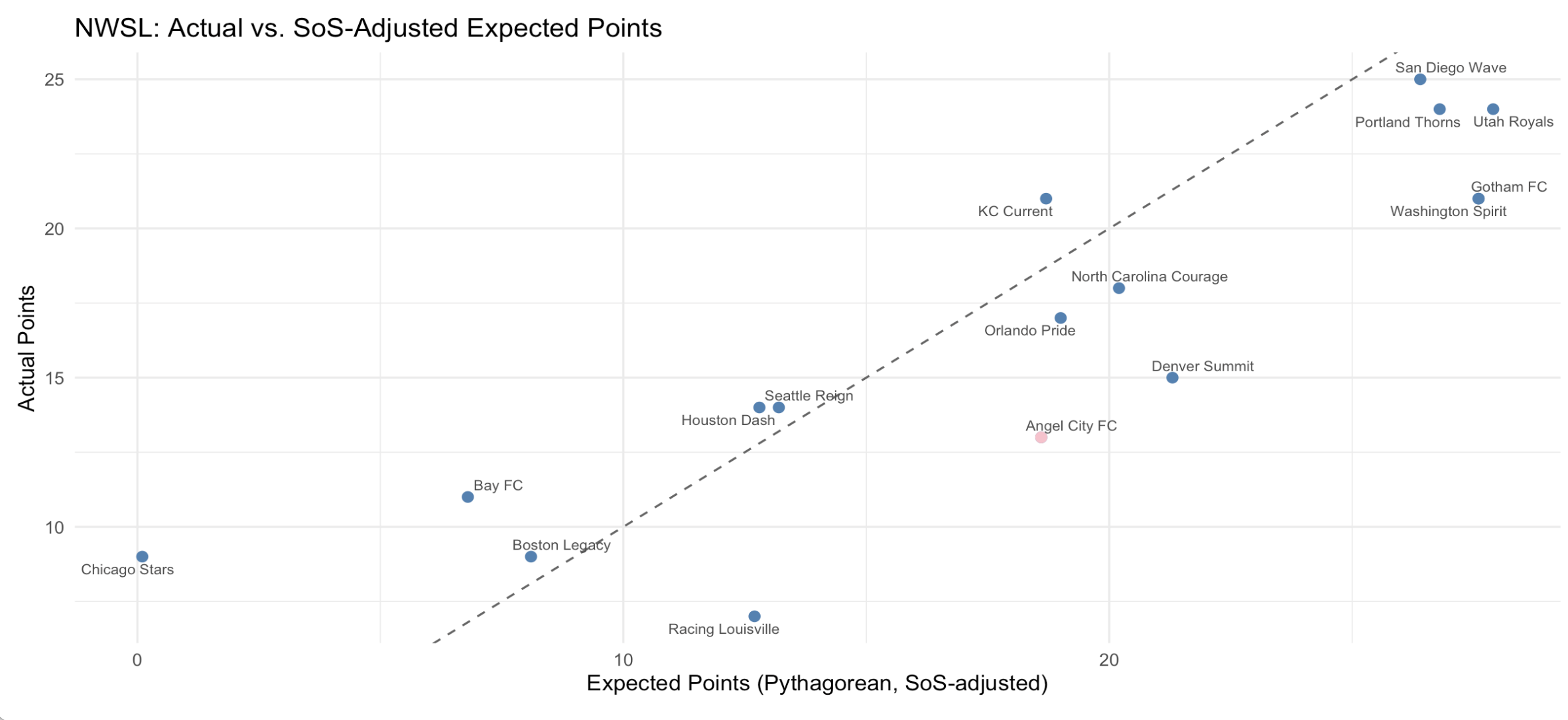
This strength of schedule (SoS) was used in two ways: 1) It added more weight to goals scored against good teams (and less against bad teams), and 2) It was used to determine the expected points, both in terms of ExpPoints to date, and in projecting the rest of the season. In essence, the model predicts a team to get fewer points against a strong opponent, and more points against a weaker one. Through trial and error, I settled on weighting the SoS at 0.25. At higher levels, it seemed to exert too much influence (for example it was saying that to date, Chicago should not have any points), while at lesser levels, it wasn’t providing enough of an influence.

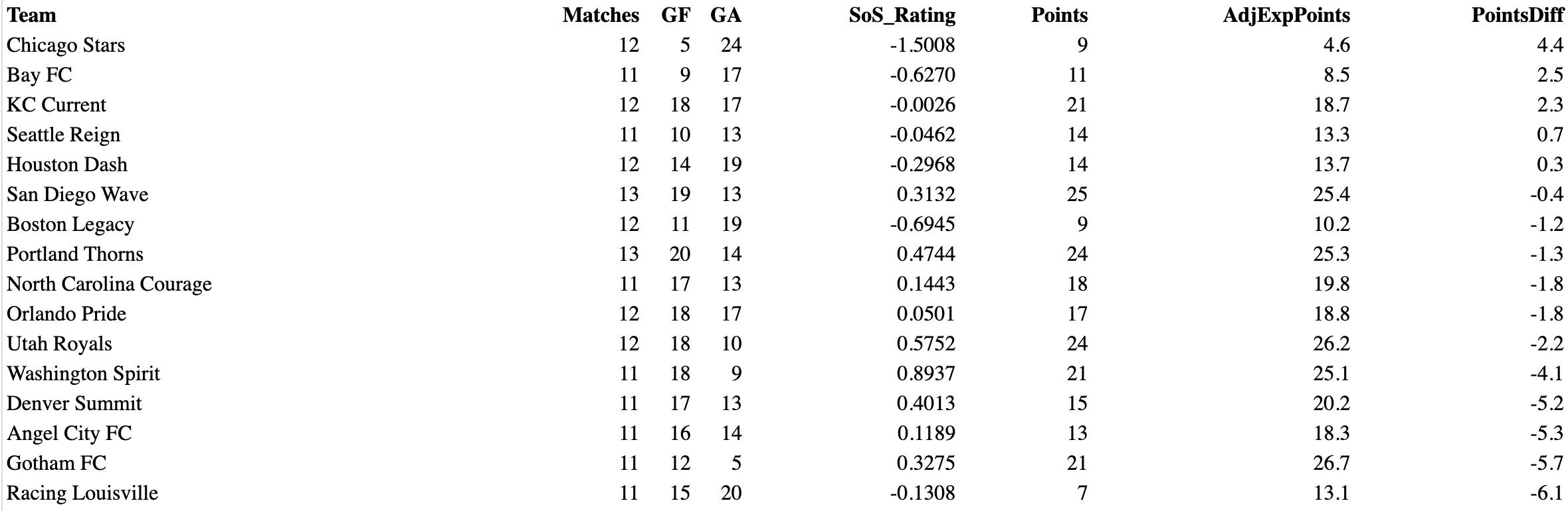
There are a few things that strike me from the table above, from an ACFC perspective. First is that Angel City’s SoS is the 8th hardest at +0.1189. This should eliminate the concerns about the big wins over Chicago and Bay skewing ACFC’s overall Goal Differential, as this model diminishes that impact. Angel City also stands out having a positive SoS, while the teams immediately around us in the table (Seattle, Houston, Bay and Boston), all have negative SoS. So even though they have similar amount of points, it has come against weaker opponents.

The second is that factoring in this strength of schedule moves Angel City’s Exp Points to 18.3 (10th place), compared to the simple model, which said 16.6 points (also 10th place). This increases the amount that Angel City was below expectation to -5.3. But the bigger thing, I think, is that Angel City is only 0.4 Exp Points behind Kansas City, but 4.6 Exp Points over Houston in 11th place. This model sees Angel City as being in the pack chasing a playoff spot, and already creating real separation from the group that compromise the teams that can already say this isn’t their year. It also shows the third largest gap between actual results and expected, indicating that performance levels were well above the record. To me, this emphasizes that Straus’ firing wasn’t justified, or at least that the front office was considering something else to be more important. But there is no question in my mind that Angel City was playing much better than their record at the break indicated.

Predictions

The second part of the model was providing predictions for the rest of the season. As stated earlier, this factors in the strength of schedule of the of the remainder of the season, and also differentiates between remaining home and away matches, by calculating home form and away form separately. Using these factors, it predicts the result of each remaining match, coming up with a final standing.

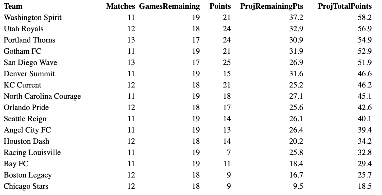
This predicts that Washington will get the Shield. Unlike the simple model, it predicts that Angel City will miss the playoffs, but that seems largely to be due to the lack of points from the first third, as it predicts only seven other teams getting more points in the remaining games. It does keep Angel City with the pack chasing a playoff spot, and maintains that there will (would be) as sizeable gap down to the next team, which it predicts to be Houston. This is the way that I had viewed Straus’ Angel City, as not quite at the top level, but on the fringes. With the coaching change, though, I don’t think this can really be viewed as the same team. We’ll have to see how they play when they come back.

Obviously there are a lot of factors that aren’t accounted for here, most especially injuries and transfers. For instance, this model doesn’t know that San Diego has Cat Macario waiting to join, but that Dudinha is our for the rest of the year. This table does feel reflective of the NWSL that I’ve been watching, however. I’ll update it after 20 games, and we’ll see how much has changed.

The full code for this can be found at my Github: goosecat95/pythagorean model

Angel City’s next game is Friday July 3 at 7p Pacific at BMO Stadium. It will be broadcast on Amazon Prime.